The Worksheet Class
The worksheet class represents an Excel worksheet. It handles operations such as writing data to cells or formatting worksheet layout.
A worksheet object isn’t instantiated directly. Instead a new worksheet is
created by calling the add_worksheet() method from a Workbook()
object:
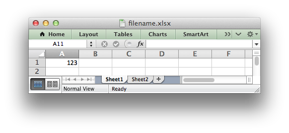
workbook   = Workbook:new("filename.xlsx")

worksheet1 = workbook:add_worksheet()
worksheet2 = workbook:add_worksheet()

worksheet1:write("A1", 123)
worksheet:write()
-
write(row, col, args) Write generic data to a worksheet cell.
Parameters: - row – The cell row (zero indexed).
- col – The cell column (zero indexed).
- args – The additional args that are passed to the sub methods such as number, string or format.
Excel makes a distinction between data types such as strings, numbers, blanks and formulas. To simplify the process of writing data using xlsxwriter the
write() method acts as a general alias for several more specific methods:
The rules for handling data in write() are as follows:
- Variables of Lua type
numberare written usingwrite_number(). - Empty strings and
nilare written usingwrite_blank(). - Variables of Lua type
booleanare written usingwrite_boolean().
Strings are then handled as follows:
- Strings that start with
"="are taken to match a formula and are written usingwrite_formula(). - Strings that don’t match any of the above criteria are written using
write_string().
Here are some examples:
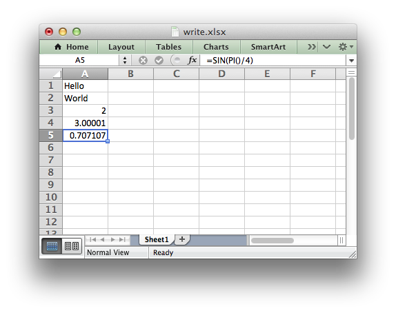
worksheet:write(0, 0, "Hello")        -- write_string()
worksheet:write(1, 0, "World")        -- write_string()
worksheet:write(2, 0, 2)              -- write_number()
worksheet:write(3, 0, 3.00001)        -- write_number()
worksheet:write(4, 0, "=SIN(PI()/4)") -- write_formula()
worksheet:write(5, 0, "")             -- write_blank()
worksheet:write(6, 0, nil)            -- write_blank()
This creates a worksheet like the following:
The write() method supports two forms of notation to designate the position
of cells: Row-column notation and A1 notation:
-- These are equivalent.
worksheet:write(0, 0, "Hello")
worksheet:write("A1", "Hello")
See Working with Cell Notation for more details.
The format parameter in the sub write methods is used to apply
formatting to the cell. This parameter is optional but when present it should
be a valid Format object:
format = workbook:add_format({bold = true, italic = true})

worksheet:write(0, 0, "Hello", format) -- Cell is bold and italic.
worksheet:write_string()
-
write_string(row, col, string[, format]) Write a string to a worksheet cell.
Parameters: - row – The cell row (zero indexed).
- col – The cell column (zero indexed).
- string – String to write to cell.
- format – Optional Format object.
The write_string() method writes a string to the cell specified by row
and column:
worksheet:write_string(0, 0, "Your text here")
worksheet:write_string("A2", "or here")
Both row-column and A1 style notation are supported. See Working with Cell Notation for more details.
The format parameter is used to apply formatting to the cell. This
parameter is optional but when present is should be a valid
Format object.
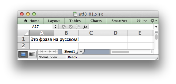
Unicode strings in Excel must be UTF-8 encoded. With xlsxwriter all that
is required is that the source file is UTF-8 encoded and Lua will handle the
UTF-8 strings like any other strings:
worksheet:write("A1", "Some UTF-8 text")
There are some sample UTF-8 sample programs in the examples directory of the
xlsxwriter repository.
The maximum string size supported by Excel is 32,767 characters. Strings longer
than this will be ignored by write_string().
Note
Even though Excel allows strings of 32,767 characters it can only display 1000 in a cell. However, all 32,767 characters are displayed in the formula bar.
worksheet:write_number()
-
write_number(row, col, number[, format]) Write a number to a worksheet cell.
Parameters: - row – The cell row (zero indexed).
- col – The cell column (zero indexed).
- number – Number to write to cell.
- format – Optional Format object.
The write_number() method writes Lua number type variable to the cell specified by row and column:
worksheet:write_number(0, 0, 123456)
worksheet:write_number("A2", 2.3451)
Like Lua, Excel stores numbers as IEEE-754 64-bit double-precision floating points. This means that, in most cases, the maximum number of digits that can be stored in Excel without losing precision is 15.
Both row-column and A1 style notation are supported. See Working with Cell Notation for more details.
The format parameter is used to apply formatting to the cell. This
parameter is optional but when present is should be a valid
Format object.
worksheet:write_formula()
-
write_formula(row, col, formula[, format[, value]]) Write a formula to a worksheet cell.
Parameters: - row – The cell row (zero indexed).
- col – The cell column (zero indexed).
- formula – Formula to write to cell.
- format – Optional Format object.
The write_formula() method writes a formula or function to the cell
specified by row and column:
worksheet:write_formula(0, 0, "=B3 + B4")
worksheet:write_formula(1, 0, "=SIN(PI()/4)")
worksheet:write_formula(2, 0, "=SUM(B1:B5)")
worksheet:write_formula("A4", "=IF(A3>1,"Yes", "No")")
worksheet:write_formula("A5", "=AVERAGE(1, 2, 3, 4)")
worksheet:write_formula("A6", "=DATEVALUE("1-Jan-2013")")
Array formulas are also supported:
worksheet:write_formula("A7", "{=SUM(A1:B1*A2:B2)}")
See also the write_array_formula() method below.
Both row-column and A1 style notation are supported. See Working with Cell Notation for more details.
The format parameter is used to apply formatting to the cell. This
parameter is optional but when present is should be a valid
Format object.
Xlsxwriter doesn’t calculate the value of a formula and instead stores the value 0 as the formula result. It then sets a global flag in the XLSX file to say that all formulas and functions should be recalculated when the file is opened. This is the method recommended in the Excel documentation and in general it works fine with spreadsheet applications. However, applications that don’t have a facility to calculate formulas, such as Excel Viewer, or some mobile applications will only display the 0 results.
If required, it is also possible to specify the calculated result of the
formula using the optional value parameter. This is occasionally necessary
when working with non-Excel applications that don’t calculate the value of the
formula. The calculated value is added at the end of the argument list:
worksheet:write("A1", "=2+2", num_format, 4)
Excel stores formulas in US style formatting regardless of the Locale or
Language of the Excel version. Therefore all formula names written using
xlsxwriter must be in English (use the following
formula translator if necessary). Also,
formulas must be written with the US style separator/range operator which is a
comma (not semi-colon). Therefore a formula with multiple values should be
written as follows:
worksheet:write_formula("A1", "=SUM(1, 2, 3)") -- OK
worksheet:write_formula("A2", "=SUM(1; 2; 3)") -- NO. Error on load.
Excel 2010 and 2013 added functions which weren’t defined in the original file
specification. These functions are referred to as future functions. Examples
of these functions are ACOT, CHISQ.DIST.RT , CONFIDENCE.NORM,
STDEV.P, STDEV.S and WORKDAY.INTL. The full list is given in the
MS XLSX extensions documentation on future functions.
When written using write_formula() these functions need to be fully
qualified with the _xlfn. prefix as they are shown in the MS XLSX
documentation link above. For example:
worksheet:write_formula("A1", "=_xlfn.STDEV.S(B1:B10)")
worksheet:write_array_formula()
-
write_array_formula(first_row, first_col, last_row, last_col, formula[, format[, value]]) Write an array formula to a worksheet cell.
Parameters: - first_row – The first row of the range. (All zero indexed.)
- first_col – The first column of the range.
- last_row – The last row of the range.
- last_col – The last col of the range.
- formula – Array formula to write to cell.
- format – Optional Format object.
The write_array_formula() method write an array formula to a cell range. In
Excel an array formula is a formula that performs a calculation on a set of
values. It can return a single value or a range of values.
An array formula is indicated by a pair of braces around the formula:
{=SUM(A1:B1*A2:B2)}.
For array formulas that return a range of values you must specify the range that the return values will be written to:
worksheet:write_array_formula("A1:A3",    "{=TREND(C1:C3,B1:B3)}")
worksheet:write_array_formula(0, 0, 2, 0, "{=TREND(C1:C3,B1:B3)}")
If the array formula returns a single value then the first_ and last_
parameters should be the same:
worksheet:write_array_formula("A1:A1", "{=SUM(B1:C1*B2:C2)}")
It this case however it is easier to just use the write_formula() or
write() methods:
-- Same as above but more concise.
worksheet:write("A1", "{=SUM(B1:C1*B2:C2)}")
worksheet:write_formula("A1", "{=SUM(B1:C1*B2:C2)}")
As shown above, both row-column and A1 style notation are supported. See Working with Cell Notation for more details.
The format parameter is used to apply formatting to the cell. This
parameter is optional but when present is should be a valid
Format object.
If required, it is also possible to specify the calculated value of the
formula. This is occasionally necessary when working with non-Excel
applications that don’t calculate the value of the formula. The calculated
value is added at the end of the argument list:
worksheet:write_array_formula("A1:A3", "{=TREND(C1:C3,B1:B3)}", format, 105)
See also Example: Array formulas.
worksheet:write_blank()
-
write_blank(row, col, blank[, format]) Write a blank worksheet cell.
Parameters: - row – The cell row (zero indexed).
- col – The cell column (zero indexed).
- blank –
nilor empty string. The value is ignored. - format – Optional Format object.
Write a blank cell specified by row and column:
worksheet:write_blank(0, 0, nil, format)
This method is used to add formatting to a cell which doesn’t contain a string or number value.
Excel differentiates between an “Empty” cell and a “Blank” cell. An “Empty” cell is a cell which doesn’t contain data or formatting whilst a “Blank” cell doesn’t contain data but does contain formatting. Excel stores “Blank” cells but ignores “Empty” cells.
As such, if you write an empty cell without formatting it is ignored:
worksheet:write(0, 0, nil, format) -- write_blank()
worksheet:write(0, 1, nil)         -- Ignored
This seemingly uninteresting fact means that you can write tables of data
without special treatment for nil or empty string values.
As shown above, both row-column and A1 style notation are supported. See Working with Cell Notation for more details.
worksheet:write_boolean()
-
write_boolean(row, col, boolean[, format]) Write a boolean value to a worksheet cell.
Parameters: - row – The cell row (zero indexed).
- col – The cell column (zero indexed).
- boolean – Boolean value to write to cell.
- format – Optional Format object.
The write_boolean() method writes a boolean value to the cell specified by
row and column:
worksheet:write_boolean(0, 0, true)
worksheet:write_boolean("A2", false)
Both row-column and A1 style notation are supported. See Working with Cell Notation for more details.
The format parameter is used to apply formatting to the cell. This
parameter is optional but when present is should be a valid
Format object.
worksheet:write_date_time()
-
write_date_time(row, col, date_time[, format]) Write a date or time to a worksheet cell.
Parameters: - row – The cell row (zero indexed).
- col – The cell column (zero indexed).
- date_time – A
os.time()style table of date values. - format – Optional Format object.
The write_date_time() method can be used to write a date or time in os.time()
style format to the cell specified by row and column:
worksheet:write_date_time(0, 0, date_time, date_format)
The date_time should be a table of values like those used for os.time():
| Key | Value |
|---|---|
| year | 4 digit year |
| month | 1 - 12 |
| day | 1 - 31 |
| hour | 0 - 23 |
| min | 0 - 59 |
| sec | 0 - 59.999 |
A date/time should have a format of type Format,
otherwise it will appear as a number:
date_format = workbook:add_format({num_format = "d mmmm yyyy"})
date_time   = {year = 2014, month = 3, day = 17}

worksheet:write_date_time("A1", date_time, date_format)
See Working with Dates and Time for more details.
worksheet:write_date_string()
-
write_date_string(row, col, date_string[, format]) Write a date or time to a worksheet cell.
Parameters: - row – The cell row (zero indexed).
- col – The cell column (zero indexed).
- date_string – A
os.time()style table of date values. - format – Optional Format object.
The write_date_string() method can be used to write a date or time string to the cell specified by row and column:
worksheet:write_date_string(0, 0, date_string, date_format)
The date_string should be in the following format:
yyyy-mm-ddThh:mm:ss.sss
This conforms to an ISO8601 date but it should be noted that the full range of ISO8601 formats are not supported.
The following variations on the date_string parameter are permitted:
yyyy-mm-ddThh:mm:ss.sss  -- Standard format.
yyyy-mm-ddThh:mm:ss.sssZ -- Additional Z (but not time zones).
yyyy-mm-dd               -- Date only, no time.
           hh:mm:ss.sss  -- Time only, no date.
           hh:mm:ss      -- No fractional seconds.
Note that the T is required for cases with both date and time and seconds are required for all times.
A date/time should have a format of type Format,
otherwise it will appear as a number:
date_format = workbook:add_format({num_format = "d mmmm yyyy"})

worksheet:write_date_string("A1", "2014-03-17", date_format)
See Working with Dates and Time for more details.
worksheet:write_url()
-
write_url(row, col, url[, format[, string[, tip]]]) Write a hyperlink to a worksheet cell.
Parameters: - row – The cell row (zero indexed).
- col – The cell column (zero indexed).
- url – Hyperlink url.
- format – Optional Format object.
- string – An optional display string for the hyperlink.
- tip – An optional tooltip.
The write_url() method is used to write a hyperlink in a worksheet cell.
The url is comprised of two elements: the displayed string and the
non-displayed link. The displayed string is the same as the link unless an
alternative string is specified.
Both row-column and A1 style notation are supported. See Working with Cell Notation for more details.
The format parameter is used to apply formatting to the cell. This
parameter is generally required since a hyperlink without a format doesn’t look
like a link the following Format should be used:
workbook:add_format({color = "blue", underline = 1})
For example:
link_format = workbook:add_format({color = "blue", underline = 1})
worksheet:write_url("A1", "http://www.lua.org/", link_format)
Four web style URI’s are supported: http://, https://, ftp:// and
mailto::
worksheet:write_url("A1", "ftp://www.lua.org/")
worksheet:write_url("A2", "http://www.lua.org/")
worksheet:write_url("A3", "https://www.lua.org/")
worksheet:write_url("A4", "mailto:jmcnamaracpan.org")
You can display an alternative string using the string parameter:
worksheet:write_url("A1", "http://www.lua.org", link_format, "Lua")
Note
If you wish to have some other cell data such as a number or a formula you
can overwrite the cell using another call to write_*():
worksheet:write_url("A1", "http://www.lua.org/", link_format)

-- Overwrite the URL string with a formula. The cell is still a link.
worksheet:write_formula("A1", "=1+1", link_format)
There are two local URIs supported: internal: and external:. These are
used for hyperlinks to internal worksheet references or external workbook and
worksheet references:
worksheet:write_url("A1",  "internal:Sheet2!A1")
worksheet:write_url("A2",  "internal:Sheet2!A1")
worksheet:write_url("A3",  "internal:Sheet2!A1:B2")
worksheet:write_url("A4",  "internal:'Sales Data'!A1")
worksheet:write_url("A5", [[external:c:\temp\foo.xlsx]])
worksheet:write_url("A6", [[external:c:\foo.xlsx#Sheet2!A1]])
worksheet:write_url("A7", [[external:..\foo.xlsx]])
worksheet:write_url("A8", [[external:..\foo.xlsx#Sheet2!A1]])
worksheet:write_url("A9", [[external:\\NET\share\foo.xlsx]])
Worksheet references are typically of the form Sheet1!A1. You can also link
to a worksheet range using the standard Excel notation: Sheet1!A1:B2.
In external links the workbook and worksheet name must be separated by the
# character: external:Workbook:xlsx#Sheet1!A1'.
You can also link to a named range in the target worksheet: For example say you
have a named range called my_name in the workbook c:\temp\foo.xlsx you
could link to it as follows:
worksheet:write_url("A14", [[external:c:\temp\foo.xlsx#my_name]])
Excel requires that worksheet names containing spaces or non alphanumeric
characters are single quoted as follows 'Sales Data'!A1.
Links to network files are also supported. Network files normally begin with
two back slashes as follows \\NETWORK\etc. In order to generate this in a
single or double quoted string you will have to escape the backslashes,
'\\\\NETWORK\\etc' or use a block quoted string [[\\NETWORK\etc]].
Alternatively, you can avoid most of these quoting problems by using forward slashes. These are translated internally to backslashes:
worksheet:write_url("A14", "external:c:/temp/foo.xlsx")
worksheet:write_url("A15", "external://NETWORK/share/foo.xlsx")
See also Example: Adding hyperlinks.
Note
XlsxWriter will escape the following characters in URLs as required
by Excel: \s " < > \ [ ] ` ^ { } unless the URL already contains %xx
style escapes. In which case it is assumed that the URL was escaped
correctly by the user and will by passed directly to Excel.
worksheet:set_row()
-
set_row(row, height, format, options) Set properties for a row of cells.
Parameters: - row – The worksheet row (zero indexed).
- height – The row height.
- format – Optional Format object.
- options – Optional row parameters: hidden, level, collapsed.
The set_row() method is used to change the default properties of a row. The
most common use for this method is to change the height of a row:
worksheet:set_row(0, 20) -- Set the height of Row 1 to 20.
The other common use for set_row() is to set the Format for
all cells in the row:
format = workbook:add_format({bold = true})

worksheet:set_row(0, 20, format)
If you wish to set the format of a row without changing the height you can pass
nil as the height parameter or use the default row height of 15:
worksheet:set_row(1, nil, format)
worksheet:set_row(1, 15,  format) -- Same as above.
The format parameter will be applied to any cells in the row that
don’t have a format. As with Excel it is overridden by an explicit cell
format. For example:
worksheet:set_row(0, nil, format1)     -- Row 1 has format1.

worksheet:write("A1", "Hello")          -- Cell A1 defaults to format1.
worksheet:write("B1", "Hello", format2) -- Cell B1 keeps format2.
The options parameter is a table with the following possible keys:
"hidden""level""collapsed"
Options can be set as follows:
worksheet:set_row(0, 20, format, {hidden = true})

-- Or use defaults for other properties and set the options only.
worksheet:set_row(0, nil, nil, {hidden = true})
The "hidden" option is used to hide a row. This can be used, for example,
to hide intermediary steps in a complicated calculation:
worksheet:set_row(0, nil, nil, {hidden = true})
The "level" parameter is used to set the outline level of the row. Adjacent rows with the same outline level are grouped together into a single outline.
The following example sets an outline level of 1 for some rows:
worksheet:set_row(0, nil, nil, {level = 1})
worksheet:set_row(1, nil, nil, {level = 1})
worksheet:set_row(2, nil, nil, {level = 1})
Excel allows up to 7 outline levels. The "level" parameter should be in the
range 0 <= level <= 7.
The "hidden" parameter can also be used to hide collapsed outlined rows
when used in conjunction with the "level" parameter:
worksheet:set_row(1, nil, nil, {hidden = true, level = 1})
worksheet:set_row(2, nil, nil, {hidden = true, level = 1})
The "collapsed" parameter is used in collapsed outlines to indicate which
row has the collapsed '+' symbol:
worksheet:set_row(3, nil, nil, {collapsed = true})
worksheet:set_column()
-
set_column(first_col, last_col, width, format, options) Set properties for one or more columns of cells.
Parameters: - first_col – First column (zero-indexed).
- last_col – Last column (zero-indexed). Can be same as firstcol.
- width – The width of the column(s).
- format – Optional Format object.
- options – Optional parameters: hidden, level, collapsed.
The set_column() method can be used to change the default properties of a
single column or a range of columns:
worksheet:set_column(1, 3, 30) -- Width of columns B:D set to 30.
If set_column() is applied to a single column the value of first_col
and last_col should be the same:
worksheet:set_column(1, 1, 30) -- Width of column B set to 30.
It is also possible, and generally clearer, to specify a column range using the form of A1 notation used for columns. See Working with Cell Notation for more details.
Examples:
worksheet:set_column(0, 0,  20) -- Column  A   width set to 20.
worksheet:set_column(1, 3,  30) -- Columns B-D width set to 30.
worksheet:set_column("E:E", 20) -- Column  E   width set to 20.
worksheet:set_column("F:H", 30) -- Columns F-H width set to 30.
The width corresponds to the column width value that is specified in Excel. It is approximately equal to the length of a string in the default font of Calibri 11. Unfortunately, there is no way to specify “AutoFit” for a column in the Excel file format. This feature is only available at runtime from within Excel. It is possible to simulate “AutoFit” by tracking the width of the data in the column as your write it.
As usual the format Format parameter is optional. If
you wish to set the format without changing the width you can pass nil as
the width parameter:
format = workbook:add_format({bold = true})

worksheet:set_column(0, 0, nil, format)
The format parameter will be applied to any cells in the column that
don’t have a format. For example:
worksheet:set_column("A:A", nil, format1) -- Col 1 has format1.

worksheet:write("A1", "Hello")             -- Cell A1 defaults to format1.
worksheet:write("A2", "Hello", format2)    -- Cell A2 keeps format2.
A row format takes precedence over a default column format:
worksheet:set_row(0, nil, format1)        -- Set format for row 1.
worksheet:set_column("A:A", nil, format2) -- Set format for col 1.

worksheet:write("A1", "Hello")             -- Defaults to format1
worksheet:write("A2", "Hello")             -- Defaults to format2
The options parameters are the same as shown in set_row() above.
worksheet:get_name()
-
get_name() Retrieve the worksheet name.
The get_name() method is used to retrieve the name of a worksheet: This is
sometimes useful for debugging or logging:
print(worksheet:get_name())
There is no set_name() method since the name needs to set when the worksheet
object is created. The only safe way to set the worksheet nameis via the
add_worksheet() method.
worksheet:activate()
-
activate() Make a worksheet the active, i.e., visible worksheet:
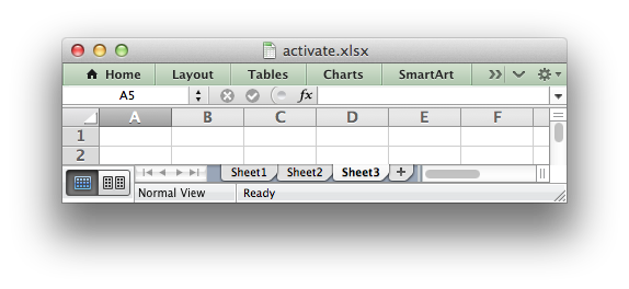
The activate() method is used to specify which worksheet is initially
visible in a multi-sheet workbook:
worksheet1 = workbook:add_worksheet()
worksheet2 = workbook:add_worksheet()
worksheet3 = workbook:add_worksheet()

worksheet3:activate()
More than one worksheet can be selected via the select() method, see below,
however only one worksheet can be active.
The default active worksheet is the first worksheet:
worksheet:select()
-
select() Set a worksheet tab as selected.
The select() method is used to indicate that a worksheet is selected in a
multi-sheet workbook:
worksheet1:activate()
worksheet2:select()
worksheet3:select()
A selected worksheet has its tab highlighted. Selecting worksheets is a way of
grouping them together so that, for example, several worksheets could be
printed in one go. A worksheet that has been activated via the activate()
method will also appear as selected.
worksheet:hide()
-
hide() Hide the current worksheet:
The hide() method is used to hide a worksheet:
worksheet2:hide()
You may wish to hide a worksheet in order to avoid confusing a user with intermediate data or calculations.
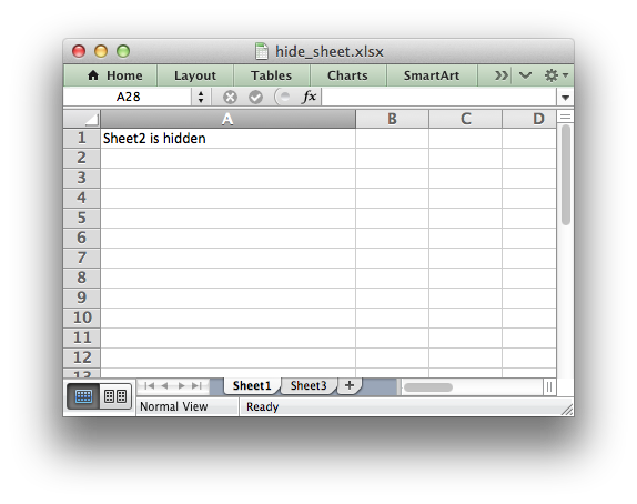
A hidden worksheet can not be activated or selected so this method is mutually
exclusive with the activate() and select() methods. In
addition, since the first worksheet will default to being the active
worksheet, you cannot hide the first worksheet without activating another
sheet:
worksheet2:activate()
worksheet1:hide()
See Example: Hiding Worksheets for more details.
worksheet:set_first_sheet()
-
set_first_sheet() Set current worksheet as the first visible sheet tab.
The activate() method determines which worksheet is initially selected.
However, if there are a large number of worksheets the selected worksheet may
not appear on the screen. To avoid this you can select which is the leftmost
visible worksheet tab using set_first_sheet():
for i = 1, 20 do
  workbook:add_worksheet
end

worksheet19:set_first_sheet() -- First visible worksheet tab.
worksheet20:activate()        -- First visible worksheet.
This method is not required very often. The default value is the first worksheet:
worksheet:merge_range()
-
merge_range(first_row, first_col, last_row, last_col, format) Merge a range of cells.
Parameters: - first_row – The first row of the range. (All zero indexed.)
- first_col – The first column of the range.
- last_row – The last row of the range.
- last_col – The last col of the range.
- data – Cell data to write.
- format – Optional Format object.
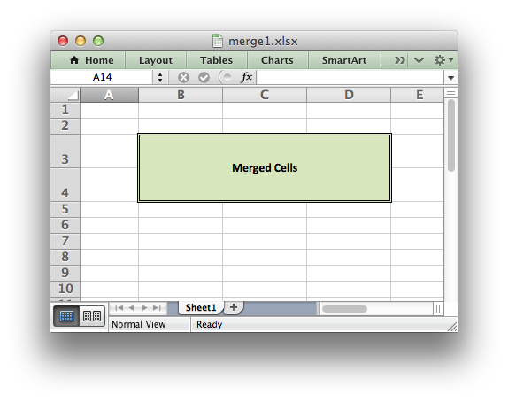
The merge_range() method allows cells to be merged together so that they
act as a single area.
Excel generally merges and centers cells at same time. to get similar behaviour with xlsxwriter you need to apply a Format:
merge_format = workbook:add_format({align = "center"})

worksheet:merge_range("B3:D4", "Merged Cells", merge_format)
It is possible to apply other formatting to the merged cells as well:
merge_format = workbook:add_format({
    bold     = true,
    border   = 6,
    align    = "center",
    valign   = "vcenter",
    fg_color = "#D7E4BC",
})

worksheet:merge_range("B3:D4", "Merged Cells", merge_format)
See Example: Merging Cells for more details.
The merge_range() method writes its data argument using
write(). Therefore it will handle numbers, strings and formulas as
usual. If this doesn’t handle your data correctly then you can overwrite the
first cell with a call to one of the other
write_*() methods using the same Format as in the merged cells.
worksheet:set_zoom()
-
set_zoom(zoom) Set the worksheet zoom factor.
Parameters: zoom – Worksheet zoom factor.
Set the worksheet zoom factor in the range 10 <= zoom <= 400:
worksheet1:set_zoom(50)
worksheet2:set_zoom(75)
worksheet3:set_zoom(300)
worksheet4:set_zoom(400)
The default zoom factor is 100. It isn’t possible to set the zoom to “Selection” because it is calculated by Excel at run-time.
Note, set_zoom() does not affect the scale of the printed page. For that
you should use set_print_scale().
worksheet:right_to_left()
-
right_to_left() Display the worksheet cells from right to left for some versions of Excel.
The right_to_left() method is used to change the default direction of the
worksheet from left-to-right, with the A1 cell in the top left, to
right-to-left, with the A1 cell in the top right.
worksheet:right_to_left()
This is useful when creating Arabic, Hebrew or other near or far eastern worksheets that use right-to-left as the default direction.
worksheet:hide_zero()
-
hide_zero() Hide zero values in worksheet cells.
The hide_zero() method is used to hide any zero values that appear in
cells:
worksheet:hide_zero()
worksheet:set_tab_color()
-
set_tab_color() Set the colour of the worksheet tab.
Parameters: color – The tab color.
The set_tab_color() method is used to change the colour of the worksheet
tab:
worksheet1:set_tab_color("red")
worksheet2:set_tab_color("#FF9900") -- Orange
The colour can be a Html style #RRGGBB string or a limited number named
colours, see Working with Colors and Example: Setting Worksheet Tab Colours for more details.
worksheet:protect()
-
protect() Protect elements of a worksheet from modification.
Parameters: - password – A worksheet password.
- options – A table of worksheet options to protect.
The protect() method is used to protect a worksheet from modification:
worksheet:protect()
The protect() method also has the effect of enabling a cell’s locked
and hidden properties if they have been set. A locked cell cannot be
edited and this property is on by default for all cells. A hidden cell will
display the results of a formula but not the formula itself. These properties
can be set using the set_locked() and set_hidden() format methods.
You can optionally add a password to the worksheet protection:
worksheet:protect("abc123")
Passing the empty string "" is the same as turning on protection without a
password.
You can specify which worksheet elements you wish to protect by passing a
table in the options argument with any or all of the following keys:
-- Default values are shown.
options = {
  ["objects"]               = false,
  ["scenarios"]             = false,
  ["format_cells"]          = false,
  ["format_columns"]        = false,
  ["format_rows"]           = false,
  ["insert_columns"]        = false,
  ["insert_rows"]           = false,
  ["insert_hyperlinks"]     = false,
  ["delete_columns"]        = false,
  ["delete_rows"]           = false,
  ["select_locked_cells"]   = true,
  ["sort"]                  = false,
  ["autofilter"]            = false,
  ["pivot_tables"]          = false,
  ["select_unlocked_cells"] = true,
}
The default boolean values are shown above. Individual elements can be protected as follows:
worksheet:protect("acb123", {["insert_rows"] = 1})
See also the set_locked() and set_hidden() format methods and
Example: Enabling Cell protection in Worksheets.
Note
Worksheet level passwords in Excel offer very weak protection. They do not
encrypt your data and are very easy to deactivate. Full workbook encryption
is not supported by xlsxwriter.lua since it requires a completely different
file format and would take several man months to implement.